Road to a Deployable Recommender System with STEM-Away

Amel Abdelraheem

Advanced Machine Learning Pathway Team @ STEM-Away

Building a production-targeted machine learning application may seem difficult, especially with the large volume of resources surrounding work in machine learning. Most people look at machine learning and think it is some sort of black magic that is able to mysteriously solve everything, this assumption then naturally develops into hesitation and confusion when it comes to taking ML outside of research labs and into production-level code.

In practice, the gap between proposed ML use cases and robust implementations of models in production environments is quite large. Often, code that is written to bootstrap ML experiments does not scale well to larger datasets, is not designed to handle predictions in real-time, does not accommodate drift in data distributions over time, and is not unit-tested for accuracy as the experiments rapidly shift. Production quality code must address these themes as well as interface with existing systems and services.

In other words, when trying to move to production we need to consider aspects beyond just modeling, when, where, and how we are getting our data, how to streamline the pipeline to ensure minimal or manageable maintenance as well as how this piece of functionality can be added and how it affects the overall system.

In this post, we will try to walk you through our journey to developing a recommender system aimed for discourse forums.

This work was done in the context of STEM-Away virtual internships - https://stemaway.com

STEM-Away

A social-impact business that provides STEM students with virtual internships. These projects span different categories with different levels of experience, one of those pathways is: Machine Learning. There are two levels of projects: Base projects (Career exploration) and advanced projects(Career Advancement).

STEM-Away also offers a preparation stage prior to the actual internships, this consists of mentor meeting, leads training and much more. People can then explore all the open projects and kind of get a feel of what the actual work will be like.

A big part of the real world experience is ambiguity and change, plans often need to be reviewed and objectives re-adjusted based on the information available. This is something we encountered early on, originally, the advanced project was set to be a drug discovery with ML project, however towards the end of the pre-phase we could tell that our cohort had many beginners with little experience in ML, which meant that a more rigorous academic route wouldn’t be the best choice, and that we will probably end up with a smaller team disconnected from the rest of the ML pathway. Thus, after many discussions with our mentor we felt it would be best to go with something more adjacent to the base ML project, which could open room for collaborations, and build a bridge between the two of us.

This was an important step for us, as it allowed us early on to be decisive and resolve early conflicts, which was a highly emphasized aspect in the STEM-Away experience.

Overview

One of the most important things to do before diving into a project is examining:

What our problem is.
Why we need to solve it.
What are the best tools available to tackle it.

When thinking about recommender systems the first thing that might come to someone’s mind is something similar to Netflix’s movies suggestions, or just your everyday YouTube feed, however those are not the only recommender systems out there. In fact, any system that tries to use user specific data - whether automatically collected or prompted to provide - in order to rank specific information and present the results back to the user is a recommender.

With the explosion of online media consumption, the need for these systems have risen and manifested in many different forms. These systems may be developed using collaborative filtering approaches (using similar user patterns for recommendations), using content based approaches (depending on the specific user’s profile and data to construct recommendations) or a hybrid of both, depending on the nature of the task and also the availability of data.

💡 Most machine learning approaches are content based approaches, in other words they use the available user data to directly make recommendations, taking a prompt and making suggestions based on that prompt falls into this category. However there are many ways to include collaborative filtering approaches for example constructing a knowledge graph and making predictions (i.e. links or nodes) by associating the patterns.

Recommender Systems For Discussion Forums

If you are a STEM student you have undoubtedly came across StackOverflow more than a few times in your student life. Most developers would also say that StackOverflow is their number one go-to place when they are stuck with something. However, if you were to go to stackOverflow and put in a simple question like: “How to print in python?” You will see that most of the suggestions you are getting are pretty far off, one possible reason for this is that these forums seem to be heavily based on tags rather than text-semantics.

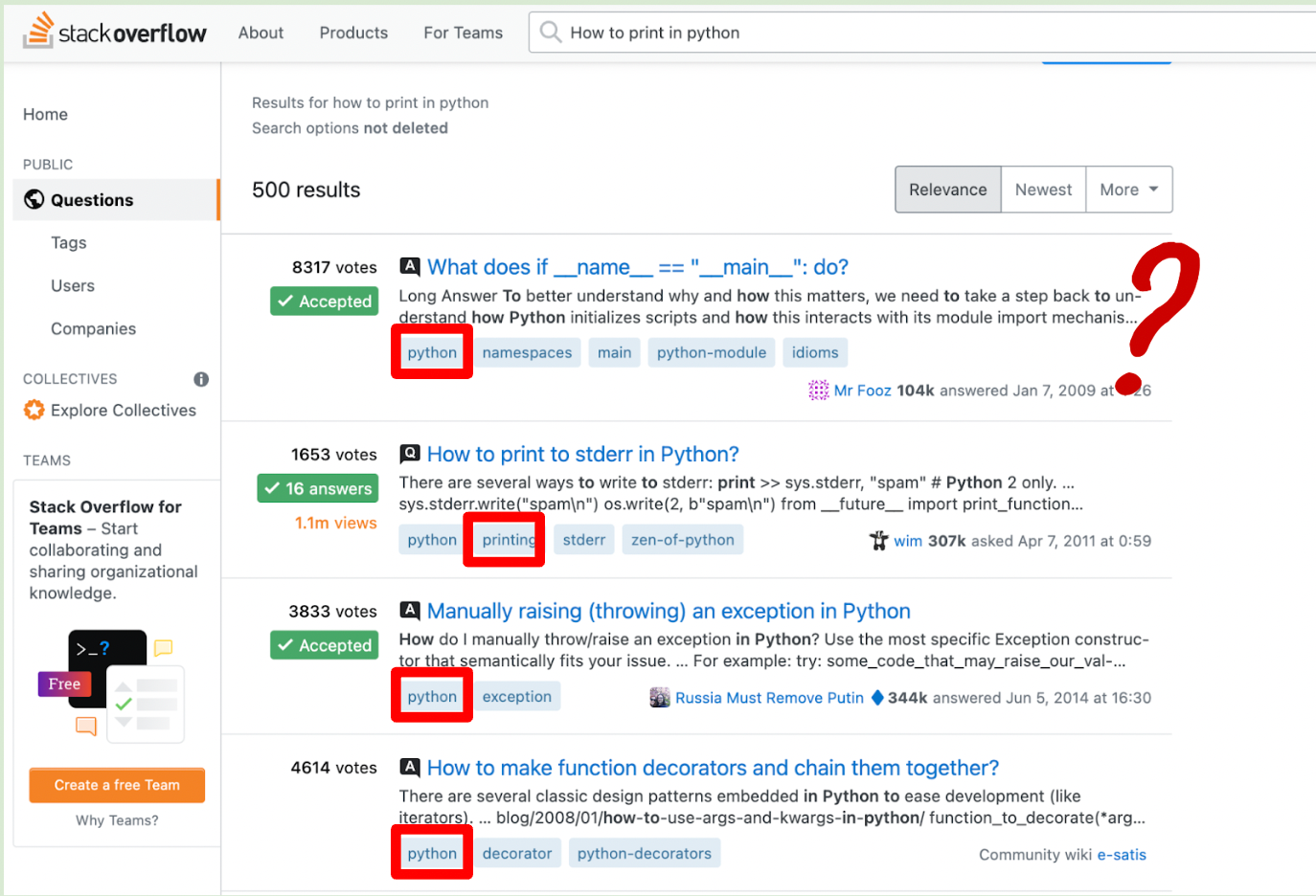
Stack-overflow’s current set-up

Admittedly however, questions are asked on Google rather than directly on stackOverflow, with the search and retrieval done entirely on Google’s end.

A similar platform to StackOverflow is Discourse which is an open source discussion platform, equipped with support for categorization and tagging of discussions, and because it’s public many communities can get their personal pages up and running by modifying the existing codes.

This means that we can’t solely rely on Google anymore and an improvement to these internal retrieval systems needs to be made , it’s also important to quickly locate and flag duplicate questions and discussions, a feature currently missing in Discourse Forums.

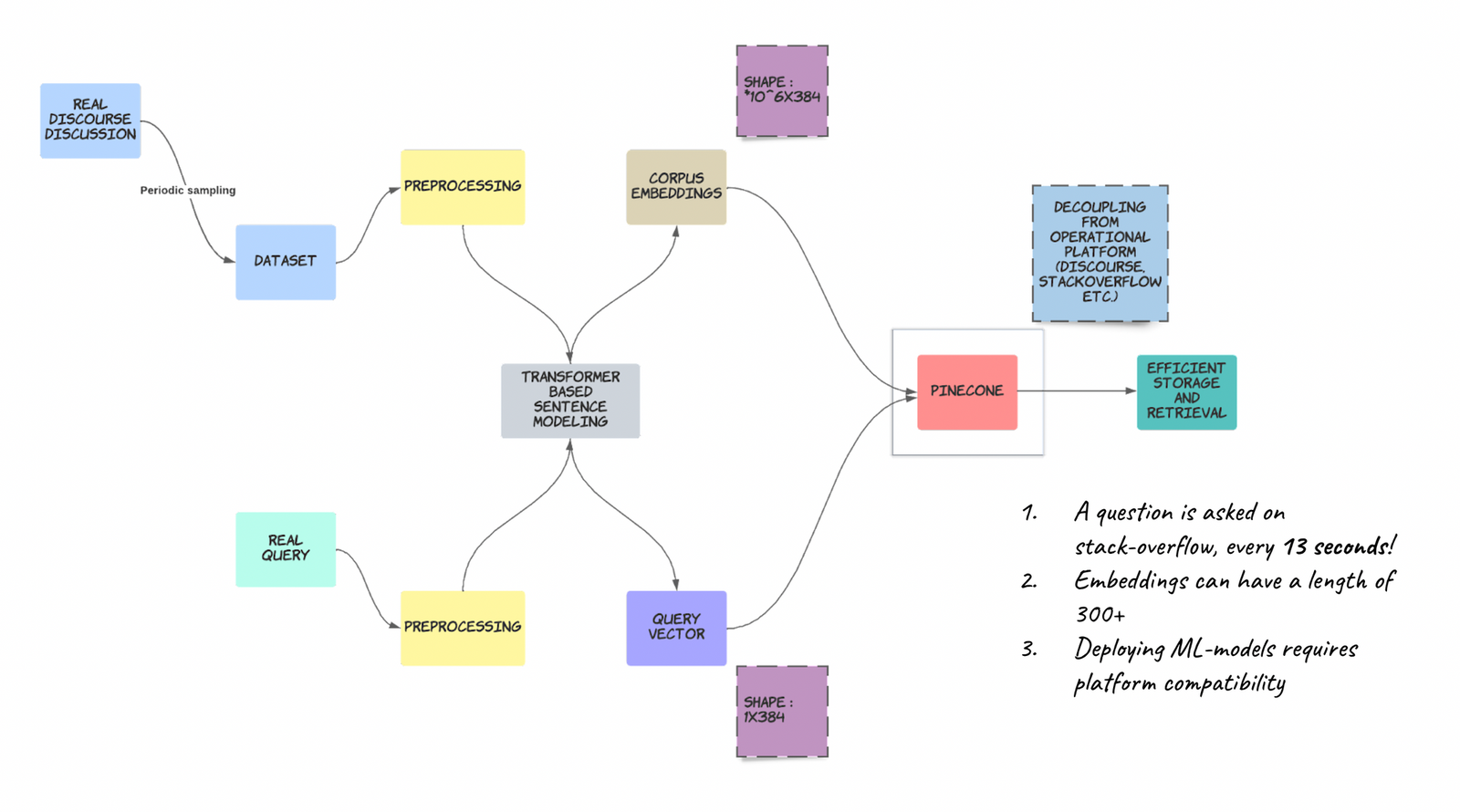
Pipeline

A schematic showing what we set out to do, different components will be explained throughout the blog-post.

Recommender System

Where to start?

Now you are probably thinking how do we start this? and the first thing to do is to break down the issue to sub-parts, to do so, we must first understand how machine learning models work.

Computers don’t really understand language like us, instead they understand numbers, so we first need to find a way to “represent” text in a way that a computer would understand, this can be done in a variety of ways, the simplest would be to use a one-hot vector to represent each word, this vector would be in the length of our vocabulary and would have one in the position of the word and zero otherwise. This approach works in theory but it would be very difficult to control the exponential growth of language (everyday new words are introduced), another problem with this approach is that it doesn’t take into account the relation between words in a sentence, for example the two sentences: “I bought you a present” and “You need to live in the present” both have the word “Present” but it means two different things!

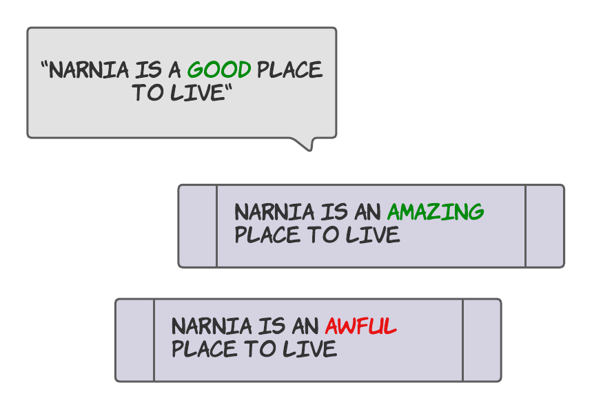
Another point to make is that one hot encoding does not preserve any notion of similarity between words, even if they are synonyms. For example below the two statements in purple will have the same distance from the our text in grey.

More approaches based on word counts and frequencies were developed in the early days of Natural Language Processing (NLP), notably TF-IDF (term frequency inverse document frequency) is good baseline for starting out, this approach relies on relating the frequency of the word and the frequency of it’s occurrence in a document/sentence, and an implementation is available in Sklearn.

Simply import Sklearn and your tf-idf vectorizer:

import sklearn
from sklearn.feature_extraction.text import TfidfVectorizer

You are ready to extract your embeddings:

tfidf = vectorizer.fit_transform([text1, text2])

output:
<2x6 sparse matrix of type '<class 'numpy.float64'>'
	with 10 stored elements in Compressed Sparse Row format>

The output of the tf-idf is a sparse matrix that contains columns corresponding to the total unique words in the two texts, and rows corresponding to each text. The cell value represents the tf-idf of that word for the specific text/sentence.

tfidf = vectorizer.fit_transform(['My short sentence for exploration', 'My shorter sentence for exploration'])
tfidf.todense()  # To transform the sparse matrix to a dense matrix

output:
matrix([[0.4090901 , 0.4090901 , 0.4090901 , 0.4090901 , 0.57496187,
         0.        ],
        [0.4090901 , 0.4090901 , 0.4090901 , 0.4090901 , 0.        ,
         0.57496187]])

Note: All Specifics of text pre-processing are omitted for the sake of simplicity, all codes can be found in our Github repo provided at the end of the post

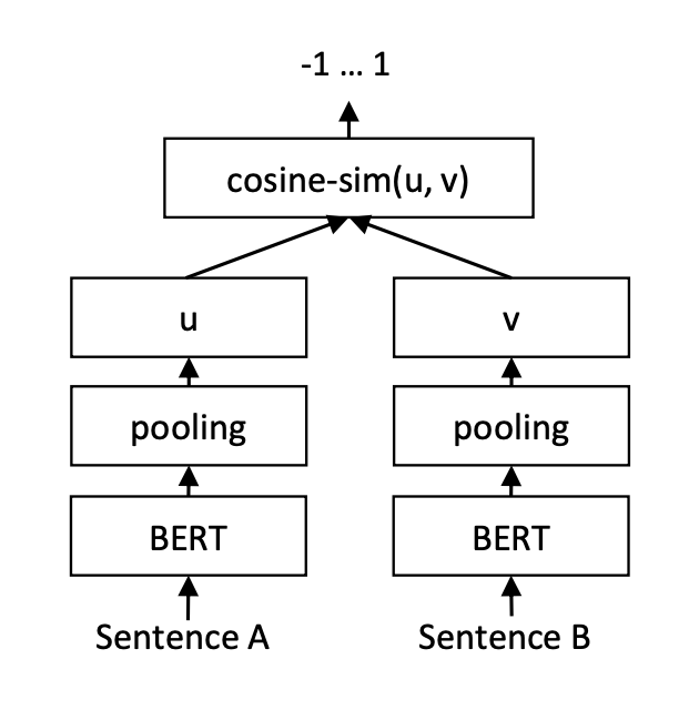
Although tf-idf can be a powerful method for some language applications, it cannot utilize contextual information. Many modern NLP applications require more flexible approaches. It wasn’t until the introduction of Transformers in 2017 (Place link) that real breakthroughs were achieved, of great interest to us is what is known as Sentence Transformers; These are powerful ML models, that take as input varying sized sentences and outputs fixed-size embeddings. These models are actually based on BERT architecture, which was a transformer based model for word embeddings that takes into account text semantics. Transformers are neural architectures that exploit the notion of attention; what a transformer does during its training is learn and assign different attentional weights to different words in a the sentence, relating to its next output.

The problem was when trying to encode a sentence with BERT you would end up with varying sized embeddings based on the sentences’ length.

Sentence-Transformers solve this by changing the BERT training schema using siamese and triplet network structures to derive semantically meaningful sentence embeddings that can be compared using cosine-similarity.

Naturally, this made sentence-transformers a very obvious choice for us. Also, Getting started with these models was also very easy thanks to HuggingFace libraries.

The following codes are an adaptation of the Wikipedia’s retrieve and rerank code available at here:

Install the sentence transformers library using pip

pip install -U sentence-transformers

2. A variety of pre-trained models exist, however we choose the following one and encoded all our sentences to get the corpus embeddings:

bi_encoder = SentenceTransformer('multi-qa-MiniLM-L6-cos-v1')
corpus_embeddings = bi_encoder.encode(passages, convert_to_tensor=True, show_progress_bar=True)

3. We also need to initialize a cross-encoder model, this model will re-rank the results we get after running similarities between the bi-encoder’s query and corpus.

#The bi-encoder will retrieve 100 documents. We use a cross-encoder, to re-rank the results list to improve the quality
cross_encoder = CrossEncoder('cross-encoder/ms-marco-MiniLM-L-6-v2')

4. Define a search function that takes your query text and returns the list of closest hits, as well as the similarity scores obtained:

def search(query, top=3):
   
    ##### Sematic Search #####
    # Encode the query using the bi-encoder and find potentially relevant passages
    question_embedding = bi_encoder.encode(query, convert_to_tensor=True)
    question_embedding = question_embedding.cuda()
    hits = util.semantic_search(question_embedding, corpus_embeddings, top_k=top_k)
    hits = hits[0]  # Get the hits for the first query

    ##### Re-Ranking #####
    # Now, score all retrieved passages with the cross_encoder
    cross_inp = [[query, passages[hit['corpus_id']]] for hit in hits]
    cross_scores = cross_encoder.predict(cross_inp)

    # Sort results by the cross-encoder scores
    for idx in range(len(cross_scores)):
        hits[idx]['cross-score'] = cross_scores[idx]

    # Output of top-k hits from bi-encoder
    
    bi_encoder_hits = sorted(hits, key=lambda x: x['score'], reverse=True)
    
    bi_list, scores = [],[]
    for hit in bi_encoder_hits[0:top]:
        bi_list.append(passages[hit['corpus_id']])
        scores.append(hit['score'])

    # Output of top-k hits from re-ranker
   
    cross_encoder_hits = sorted(bi_encoder_hits, key=lambda x: x['cross-score'], reverse=True)
    cross_list, scores_cross = [], []
    for hit in cross_encoder_hits[0:3]:
        cross_list.append((passages[hit['corpus_id']]))
        scores_cross.append(hit['cross-score'])
    return bi_list, cross_list, scores, scores_cross

5. In order to get a sense of our models performance we need to compute some sort of metric, to do so we will define a function that takes a list of queries and computes the top-k hits for them:

def compute_hits(embeddings, questions_list, model = 'cross', top=3):
  hits_dict = defaultdict(lambda: 0.0)
  for idx, question in enumerate(questions_list):
    hits = []
    bi_hits, cross_hit, bi_scores, cross_scores = search(question, top=top)
    if model == 'bi':
      hits_dict[idx] = (bi_hits, bi_scores)
    else:
      hits_dict[idx] = (cross_hit, cross_scores)
  return hits_dict

hits = compute_hits(corpus_embeddings, query_list,top=5)

6. Next we define an evaluation function to compute various metrics, i.e accuracy, sensitivity and specificity

def evaluate(list_hits, list_questions, labels):
  counts, length, TP, FP, TN, FN = 0,0,0,0,0,0
  TP_score, FP_score, TN_score, FN_score = [], [], [], []
  for idx, q in enumerate(list_questions):
      length +=1
      if labels[idx] == 1 and q in list_hits[idx][0]:
        counts+=1
        TP+=1
        # TP_score.append(list_hits[idx][1][])
      if labels[idx] == 0 and q not in list_hits[idx][0]:
        counts+=1
        TN+=1
      if labels[idx] == 1 and q not in list_hits[idx][0]:
        FN+=1
      if labels[idx] == 0 and q in list_hits[idx][0]:
        FP+=1

  accuracy = (counts/length)*100
  sensitivity = TP/(TP+FN)
  specificity = TN/(TN+FP)
  FPR = 1-specificity
  return accuracy, sensitivity, specificity, FPR, TP,TN,FP,FN

accuracy, sensitivity, specificity, FPR , TP, TN, FP, FN= evaluate(hits, query_list,labels)

At this stage we had a good system that uses the text semantics to compute similarities. We now have meaningful numeric representations, but updating, accessing, and computing on these representations is extremely inefficient in practice. For our a dataset of just 800 samples, it takes the system 42 seconds to process (Extremely slow!)

The next question on our minds was how do take this work and transform it into something production ready?

Moving from Colab to API-calls; Pinecone.io

So far most of work has been hosted on a Colab notebook, but what happens when our data is no longer in the lengths of thousands, rather hundreds of thousands. How do we manage this increasing volume and how do we adapt our models in a way that would not be affected by this not only in terms of storage but also speed.

One might think that hosting the data on a cloud database and calling it from there every time there is a query/question being asked might solve the problem, unfortunately even if we are able to do that the required compute to handle this large dataset will pose an added expense to these hosting platforms, additionally naively running these comparisons can become very slow and one would need to wait at least 15mins just to get their recommendations, obviously no one wants to wait that long for a simple answer.

All of this means, we need to approach the problem from more advanced angles, luckily for us this has already been done (and is continuously maintained) by PineCone.io.

Pinecone makes it easy to build high-performance vector search applications. It’s a managed, cloud-native vector database with a simple API and no infrastructure hassles.

What really drew us to pinecone is how simple it is to get started with it, with a few line lines of code you can have a fully operational database manager as well as a vector search engine. this means that you no longer need to run vector comparisons on your own, Pinecone will do it for you, in a fast and highly optimized way. Pretty cool if you ask us!

To get started we first need to create an account on Pinecone, once that is done we move back to our codes and install the Pincone client:

!pip install -qU pip pinecone-client

2. Next we need to import pinecone and set up our API Key (this can be found on your Pinecone’s console)

import pinecone
import os

api_key = 'f158288a-05ab-4c9f-8674-4a23758efffe'
pinecone.init(api_key=api_key, environment='us-west1-gcp')

3. We now need to create an index that would be used to host our data (the 384 is the dimension of our embeddings, this may change depending on which model you end up choosing)

index_name = "stem-away"
dimensions = 384
pinecone.create_index(name=index_name, dimension=dimensions)
index = pinecone.Index(index_name=index_name)

4. To uspert/upload the data we need to define a batching function, since our data is quite large and Pinecone has a limit on the size of data you can upsert at once

import itertools

def chunks(iterable, batch_size=100):
    it = iter(iterable)
    chunk = tuple(itertools.islice(it, batch_size))
    while chunk:
        yield chunk
        chunk = tuple(itertools.islice(it, batch_size))

for batch in chunks(zip(vectors_df.id, vectors_df.vector)):
    index.upsert(vectors=batch)

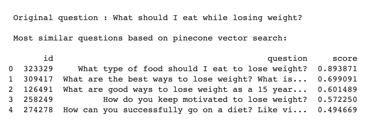
5. Let’s do some querying!

query_results = [index.query(xq, top_k=5) for xq in query_embeddings.tolist()]

You now have a fully hosted database with vector search capabilities through API Calls.

We also mentioned that Pinecone let’s introduce hybrid searches based on meta-data/filters in addition to the vector search, this can simply be done by upserting the tags/tokens along with each vector in our corpus:

upserts = []
for (id, embedding, tokens) in zip(vectors_df.id, vectors_df.vector, cleaned_tags):
    upserts.append((str(id), embedding, {'tokens': tokens}))

for batch in chunks(upserts):
    index.upsert(vectors=batch)

filters = ['python', 'Programming']
query_results = index.query(xq, top_k=5, filter={
    'tokens': {'$in': filters}})

Alluding back to our comment on speed; Pinecone is able to run the same vector search in just 3.39 seconds, which is more than x10 as fast!

Future Considerations

Fine-Tuning and customization: Getting the data Right

Although pre-trained models give good results, better results can be archived with some fine-tuning .Pre-trained models rely on the pre training corpus to contain the majority of the relevant signal for a specific problem. By fine-tuning, we can leverage the large pre-training dataset and generalized parameters, while also injecting signals that are highly specific to our problem. We can have the best of both worlds: relatively low volumes supervised data labels and training time, and a custom model that extends upon the foundation laid by the highly general and expressive pre trained model.

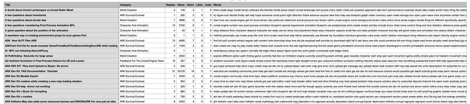
To do this we need to get data directly from the discourse forums and figure out a way to annotate them in such a way that we can run our fine-tuning. However, initial exploration for the fine-tuning was carried and explained in the following section.

💡 Note: This web scraping is Courtesy of our exploratory teams, detailed codes can be found on their github repo: link. we would limit our discussion to the general idea and how we used this data in our pipeline.

As you have seen we have two neural architectures present in our pipeline: Bi-encoder (to compute initial similarities) and a Cross-encoder (producing a finer grained results), below we will explain how to fine-tune the cross-encoder architecture:

First we need to create a list of training samples along with their labels, that contains InputExample objects, as this is what BERT-based models expect their input to be

train_samples = []
  for idx, row in train_data.iterrows():
     train_samples.append(InputExample(texts=[row['text_1'], row['text_2']], label=int(row['label'])))
     train_samples.append(InputExample(texts=[row['text_2'], row['text_1']], label=int(row['label'])))

2. We then transform this data to a Dataloader object, for ease of batched training.

train_dataloader = DataLoader(train_samples, shuffle=True, batch_size=16)

3. Next, you just need to fit/train the model and specify a path to save your weights, this is because in some cases you are not able to carry the full training in one setting, the only thing to take note of in this case is that you will load your model parameters instead of directly using the pre-trained weights.

model.fit(train_dataloader=train_dataloader,
              epochs=num_epochs,
              warmup_steps=warmup_steps,
              output_path=model_save_path)

Data Annotation

Although we were unable to perform annotation on the scraped data given our timeframe, one plausible approach would be to develop a streamlit application that would take different pairs of questions and present them to a user for labeling. This would help us construct a dataset that is identical in structure to the Qoura dataset and that is forum-specific, which means fine-tuning using this dataset would have a higher chance at improving the recommendations our system would produce in a given forum/community.

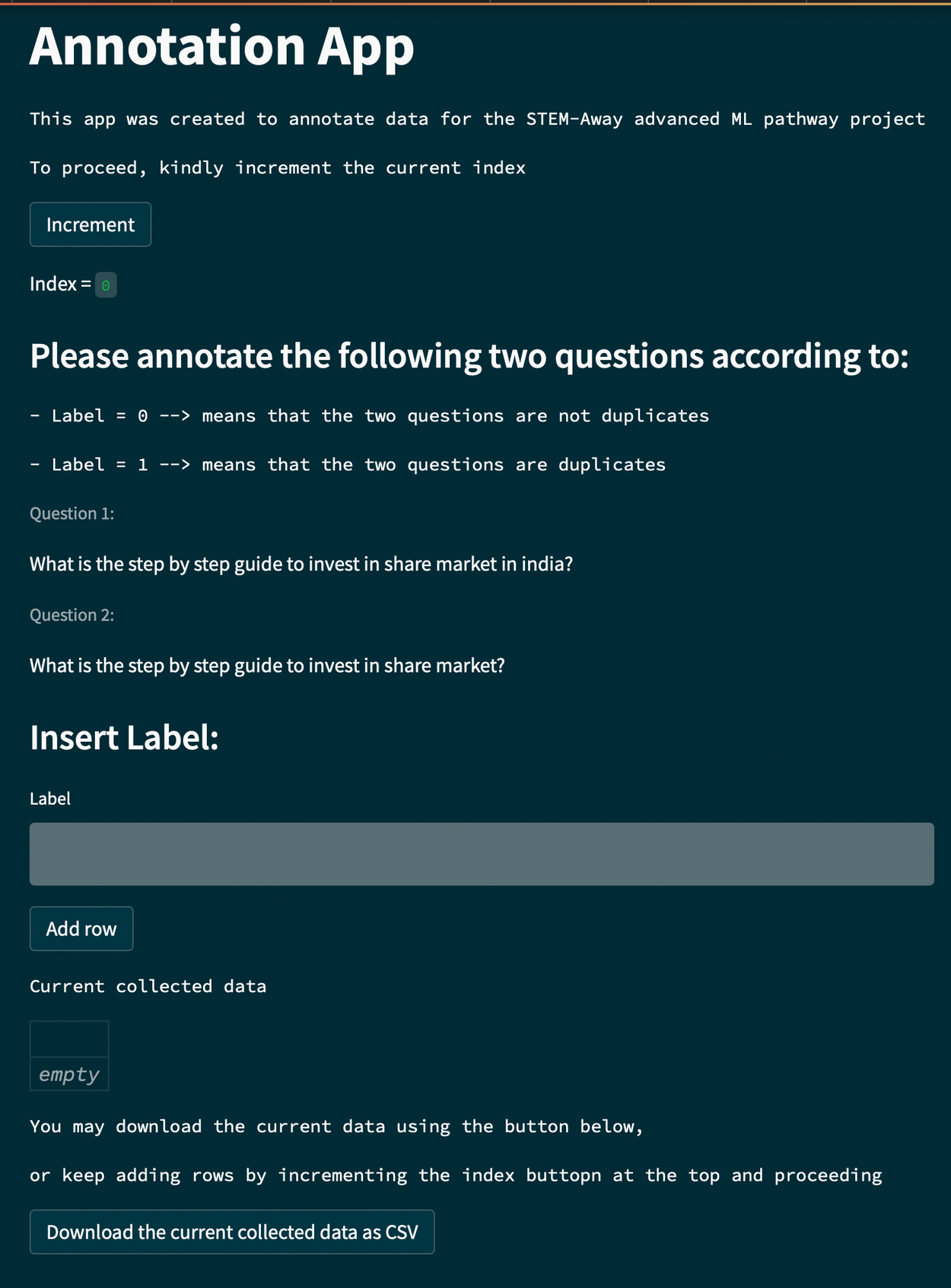
Another interesting idea would be to use TF-IDF modeling to nominate possible question pairs, for example pairs having a similarity score above a specific threshold would be displayed via the app for user labeling. However, due to the huge of volume of the dataset and the limited available existing similar pair, not many valuable candidate pairs were produced.

Closing thoughts

Building a real-world system is never easy; the data is not clean, the models are too big or too slow, and a high (or low!) accuracy on a test-set has nothing to do with live performance. However many solutions exist and many tools can be incorporated to get to that finish line. Just because a journey isn’t smooth doesn’t mean it will be a failure, a lot can be done when a group of people come together to do it, so have fun and enjoy the ride!

Special Thanks:

I would like to extend a special thanks to our mentor Colin Magdamo, who supported us beyond just this internship, but in every capacity presenting itself.

To Debaleena Das founder of STEM-Away, your spirit and constant passion made us feel nurtured and motivated to keep pushing ourselves.

Authors:

Primary author: Amel Abdelraheem. Contributions by: Sakayo Toadoum Sari, Vedant Tewari

Advanced Machine Learning Pathway Team @ STEM-Away.